Prettifying Rasters & Geoprocessing

An overview about making a typical hillshaded raster map from a Digital Elevation Model. In this post, I will also elaborate on raster stylings and useful geoprocessing functions available in QGIS, and use the qgis2threejs plugin to generate web-exportable 3D map visualizations.

Let’s try to get more raster content here. Raster maps are usually more troublesome to manage than vector maps, due to the typically large data size of raster data. However, the amount of detail easily achievable in a raster map often overshadows vector maps trying to visualize similar landscapes. Simply put, it is often not feasible to trace out the points, lines and polygons to symbolize features in elaborate landscapes. Raster maps allow you to showcase such highly detailed maps, and only be limited to output resolution. For further reading check out the QGIS documentation’s Introduction to GIS.

The following will be based off a spatial analysis and geoprocessing tutorial from Mastering QGIS by Packt Publishing, which is an excellent guidebook about many advanced QGIS functionalities.

Raster Analyses in QGIS using GRASS

Additional spatial analysis tools are available in QGIS, through integration with GRASS GIS, SAGA, GDAL and other third-party providers. Although QGIS includes quite a few algorithms natively, the algorithms available through those other powerful open source platforms extend spatial analysis capabilities seamlessly. Looking to shade relief? Type that into the Processing Toolbox and you can choose from r.relief from GRASS, or Color relief from GDAL. QGIS has its own hillshade tool, and it can be found with a bit of navigating in the menu toolbar (Raster > Analysis > DEM. Hillshade is the default option).

Our Tutorial Question

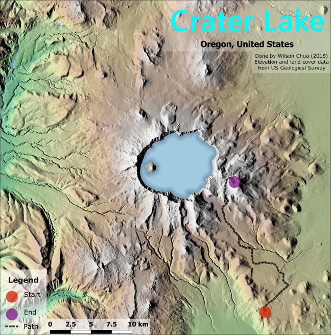
The problem statement offered by Mastering QGIS is to calculate the Least Cost Path for a hypothetical rescue team to reach a stranded hiker in Crater Lake National Park, Oregon. The processing algorithms used include the GRASS tools r.slope.aspect, r.recode, and r.cost, plus Least Cost Path from SAGA. The tutorial also makes use of the Crater Lake National Parks’s elevation and land use data from USGS.

R.slope.aspect calculates the slope, which adds to the cost. Our rescue team definitely will not appreciate steep slopes on their way to the hiker.

R.recode reclassifies our land use data as cost, using a provided reclassification table. In short, it takes the land use and assigns a cost of traversing through that area based on that table. For example while urban areas can be assigned a low cost value of 1, forests may be assigned a higher cost value of 50, as the rescuers would prefer not to bash through vegetation. If traversing across water is not feasible, it can always be assigned an unreasonable cost value, which was in this case 1000.

QGIS’s native map calculator is then used to “add” our two cost layers together into a single, combined layer. This was just to showcase the flexibility we have to switch between our platforms.

R.cost then evaluates the cumulative costs from the combined layers. The output is then applied to SAGA’s Least cost path algorithm, which is also given two point layers containing the Start Point of our rescue team and the End Point where our hiker is stranded. It generates the path as a line in a vector layer.

Prettifying the Raster

The primary option for styling rasters are colour schemes, and well-known options for topographic and elevation maps are the cpt-city colour ramps. The raw elevation map doesn’t give much semblance of topography at first glance, however. This is where is hillshade map from r.relief comes in. By setting the layer blending mode under layer styles to multiply and adjusting the colour properties (brightness, saturation, contrast) as you deem fit, we can achieve a well balanced hillshaded map.

Output Map

As of now (Feb 2018) QGIS has an experimental SVG export. However, the layer styles do not export with their blending modes, and the resultant SVG has to be further processed with a vector graphics editor. I used Inkscape for the following map. As you can see I am not able to achieve the same blending I could in QGIS.

Viewing in 3D

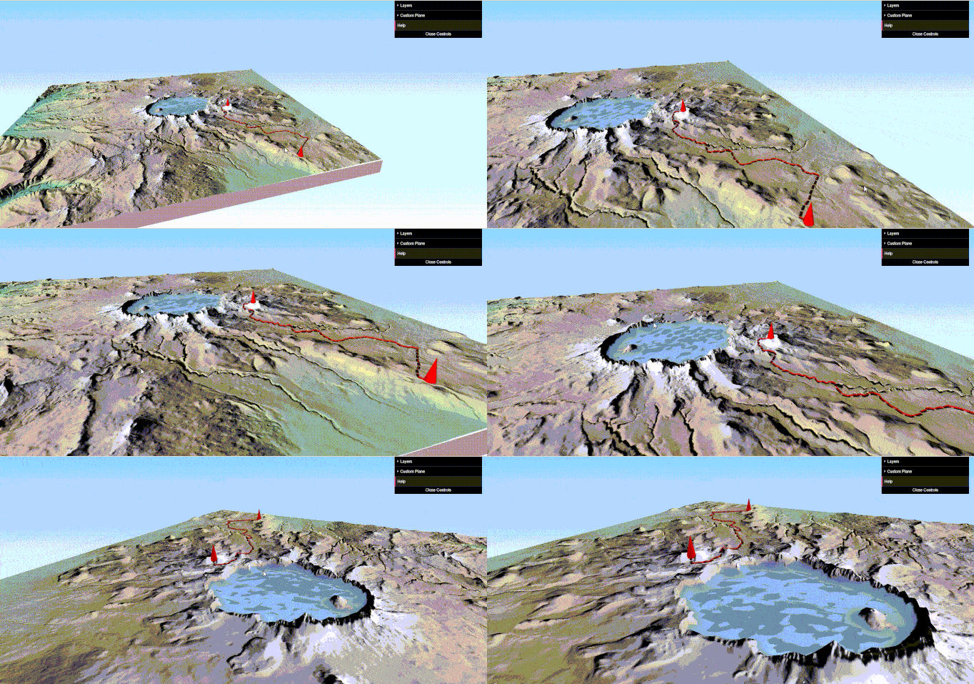
QGIS2threejs is an excellent plugin to view elevation data in 3D. The map is viewable through stunning angles offered by WebGL.

You can view the full graphic here.