Road-Graph Neural Networks

It’s been a while since my last post! Since then, I’ve completed a degree in Computing, with a slight focus towards data analytics modules. For my final year project (link to my paper), I investigated a potential synergy between Space Syntax - graph theory applied to road networks, and Graph Neural Networks, and in doing so developed a simple pipeline for machine learning on road networks using GNNs. This post serves as an introduction on how to set up such a pipeline in Python.

Introduction

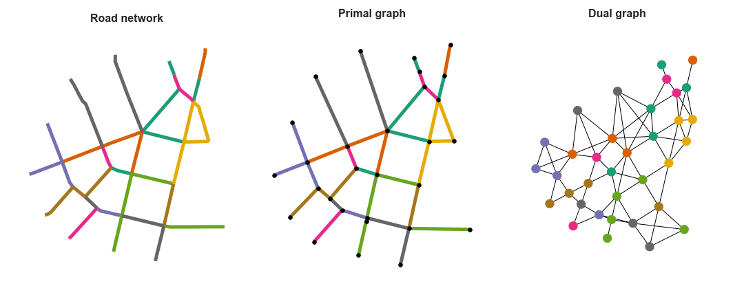
Road networks form natural graphs, with the straightforward representation of roads as edges between intersection points. However, another representation is the dual or line graph: where roads themselves are nodes and edges represent intersections between roads. This diagram depicts the difference between the two representations, using the reference street lines on the left:

Machine Learning on Graphs

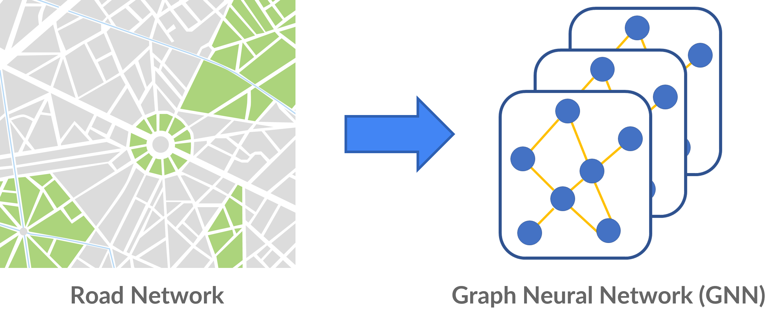
Graph-structured data are ubiquitous in data analytics, ranging from social networks to biological molecules. To learn from such structures, researchers in graph representation learning developed Graph Neural Networks (GNNs). GNNs make use of aggregation operators to generate embeddings for nodes, edges and even whole graphs. These embeddings can then be used as input for downstream tasks such as node classification, regression, and even link prediction.

With their recent explosion in popularity, there are a host of tutorials online introducing graph representation learning. So rather than reinvent the wheel, let me link some ones that I’ve found useful in my research.

• A Gentle Introduction to Graph Neural Networks by Google
• Theoretical Foundations of Graph Neural Networks by Petar Veličković

Graph Learning on Road Networks

With the advent of large georeferenced urban datasets, including open street datasets, there are several use cases that stand to benefit from GNNs.

• Traffic Prediction: This is the most popular use case, a classic example being the ETA predictor used in Google Maps.
• Completing Open Data: Most open street datasets are incomplete, often coming with missing fields such as speed limits especially in rural areas. A model can help assign the most likely speed limit classifications based on computable attributes of the road, such as its length and width.

Caveat: GNNs are imperfect

Generally, GNNs are advantageous when the target variable exhibits similar values over neighboring nodes (spatial homophily). For example, traffic volume on a single road is majorly affected by its connecting roads, and as such a road with high traffic is likely to be connected with roads of similarly high traffic.

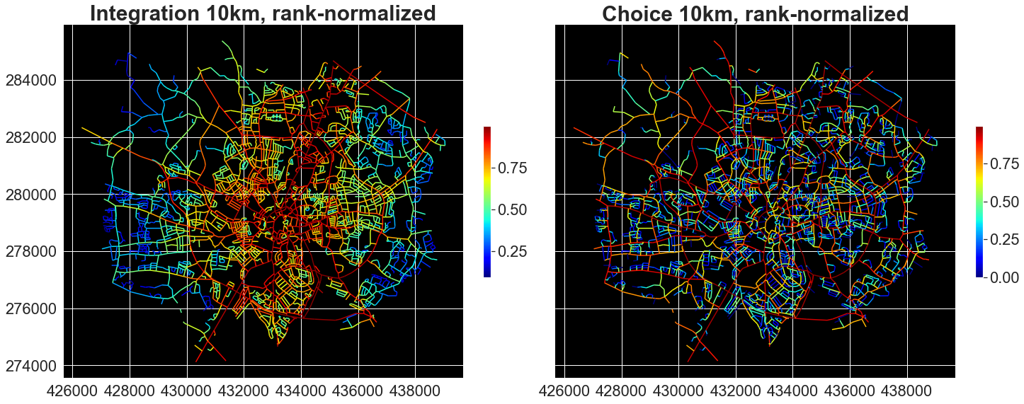
GNNs do not, however, perform as well on volatile features. For example, choice, or betweenness centrality, is commonly used in Space Syntax to measure the through-movement connectivity of roads. As such, it can exhibit drastic differences between adjacent roads e.g. a sliproad connecting to a major highway.

In my project, I discovered that GNNs do not in fact work well as a function approximator for choice, with the likely reason being this breach of the spatial homophily assumption. As such, please consider whether your study really stands to benefit from GNNs! And always, always use a standard feed-forward neural network (multilayer perceptron) as a baseline.

Graph Learning on Road Network Data

Getting Road Network Data

Existing .shp or .gpkg data can be read by geopandas, a library built for manipulating spatial data. geopandas deals with GeoDataFrames: tables containing rows that store individual geometries e.g LineStrings and Polygons. From here, there are a few options for converting GeoDataFrames of LineStrings into networkx Graphs that can be processed by popular graph learning libraries.

• gdf_to_nx from momepy. This function is capable of converting to both primal and dual graph representations.
• utils_graph.graph_from_gdfs from osmnx.

Alternatively, one can download data from OpenStreetMap directly as networkx Graphs via osmnx’s graph module.

import osmnx as ox

place = "Cambridge, England"
osmnx_buffer = 10000 # in metres
g = ox.graph.graph_from_place(place, buffer_dist=osmnx_buffer)
g = ox.projection.project_graph(g)

Preprocessing

For some cases, you might want to simplify the network by removing interstitial nodes: nodes of degree 2 that only exist to denote the road’s geometry.

The data attributes of the constituent road segments would have to be aggregated somehow, such as by taking the sum or maximum, or the mode for categorical data. All this can be done using momepy’s remove_false_nodes, which I have extended here to perform said aggregation.

Of course, these decisions will have a large impact on input data: consider which aggregations makes sense in the context of the prediction objective. For example in my project, I found out that taking the minimum of Space Syntax features slightly augments the output model’s prediction accuracy.

Converting networkx Graphs to PyTorch Geometric Data objects

I used PyTorch Geometric, a library for graph learning built upon the popular pytorch framework. PyTorch Geometric’s main advantage over other graph learning libraries is that it includes implementations of many recently developed models in the literature, making it easy to incorporate them and try them out for research. Other popular libraries to consider include Deep Graph Library (DGL), and Spektral for folks that prefer Tensorflow/Keras.

PyTorch Geometric also includes a utility, from_networkx, to convert networkx Graphs into its Data objects which can then be processed directly or loaded into DataLoaders. However depending on the road graph representation, you might have to perform feature pooling: take a look at process_primal_graph and process_dual_graph over in my data loading library for an example. The following function is an adapted process_primal_graph that performs edge feature pooling.

def process_primal_graph(g, feature_fields=[], agg='mean'):
    """
    Takes features from adjacent edges and aggregates them to form the node attribute

    Args:
        g (networkx.Graph or networkx.DiGraph): A networkx graph.
        feature_fields (List[str] or all, optional): The edge attributes to
            be pooled to form node attributes.
        agg (str): One of 'mean', 'sum', 'max' or 'min'. Aggregation is handled by
            `apply_arg`.

    """
    # ignore coordinate features (added independently)
    coord_feats = ['x', 'y', 'lng', 'lat']
    feature_fields = remove_item(feature_fields, coord_feats)
    
    for node, d in g.nodes(data=True):
        # get attributes from adjacent edges
        new_data = {field:[] for field in feature_fields}
        for _, _, edge_data in g.edges(node, data=True):
            for field in feature_fields:
                new_data[field].append(edge_data[field])
        
        if not return_nx:
            d.clear()
        # take the sum/mean of the collected attributes
        for field in feature_fields:
            d[field] = apply_agg(new_data[field], agg)
        
        # encode node coordinate as feature
        d['x'], d['y'] = node
        d['lng'], d['lat'] = node
    
    for u, v, d in g.edges(data=True):
        # encode edge information for later indexing
        d['u'] = u
        d['v'] = v
    return g

Once you have your Data objects, we can finally begin training. Check out PyTorch Geometric’s extensive documentation how to conduct further analysis, as well as their multitude of different state-of-the-art GNN implementations.

Or, check out my research repository for Jupyter Notebooks that showcase actual training loops. Fair warning though, the code gets hairy with all the different models I was testing. If you are interested, please refer to my paper for more information on the tasks that were performed.

Closing Thoughts

GNNs do hold a lot of promise for machine learning with road network data. Yet as with most machine learning tasks, only good data would give quality insights. And while there are quite a few open road network datasets out there, most are based on publicly-maintained fields that may contain inconsistencies.

Still, I hope that this post has served as a good introduction! Let me know if you have any feedback; my contacts can be found from the sidebar.